Quick-start guide

This guide introduces some of the main features of VRE Language through simple examples and use cases. The examples shown are built and processed using the Scientific Computing Language (SCL) and the texts command line tool. For simplicity and speediness the guide employs a local file as mock database, completely removing the overhead related to database server setup.

Installation and mock database setup in few minutes

The instructions for the quick installation and local database setup are:

Create a new python environment with, at least, python 3.9 and activate it;

Install the VRE Language with the mongomock extra:

python -m pip install --upgrade pip
python -m pip install "vre-language[mongomock]"

Setup the local file for the mock database by entering the following commands:

mkdir -p ~/.fireworks
echo MONGOMOCK_SERVERSTORE_FILE: $HOME/.fireworks/mongomock.json >> ~/.fireworks/FW_config.yaml
echo '{}' > ~/.fireworks/mongomock.json
lpad reset

Done. Now we can start using the VRE Language package.

Hello textS from the interactive session

The simplest way to use the SCL is through the texts session command line interface (CLI), initiated with the command:

~>$ texts session
Input > 

NOTE: The first time the texts session command is used, the program will ask to create a resource configuration file:

Resource configuration /home/.fireworks/res_config.yaml not found.
Do you want to create it?
Yes(default) | No | Ctrl+C to skip:

It is recommended to accept the automatic creation of the res_config.yaml file.

The texts session command creates an empty model that can be extended interactively by adding statements, for example our first print statement:

Input > print('Hello textS')
Output > 'Hello textS'

Next we can add some variable statements to the model. Remember that every new statement will add a new node to the model’s workflow:

Input > var1 = 1
Input > var2 = 2
Input > var3 = var1 + var2
Input > print(var3)
Output > n.c.

Notice how the Hello textS string is printed, but instead of the value of var3 it shows n.c. (not computed) because the print statement contains a reference to var3 as parameter. Parameters that do not contain references are always evaluated as soon as they are used in print statements.

By default, the texts session will not perform evaluation of references. Evaluation can be turned on in two ways:

Using the --autorun | -r flag when initiating a texts session.
Entering the %start magic command in a running session.

The evaluate-all policy is chosen by default and evaluation of all references is activated. Details about execution modes, evaluation policies, and operation blocking are available in the documentation. All available options for texts session can be displayed with the --help | -h flag.

Before returning to our model, we can introduce the %hist magic command, which prints all persistent statements together with metadata about their latest update and current state. Now we can follow the state of the model before and after activating evaluation:

Input > %hist
WAITING    2024-06-20T16:18:56+02:00 var1 = 1
WAITING    2024-06-20T16:19:08+02:00 var2 = 2
WAITING    2024-06-20T16:19:17+02:00 var3 = var1 + var2
Input > %start
Input > print(var3)
Output > 3
Input > %hist
COMPLETED  2024-06-21T18:54:05+02:00 var1 = 1
COMPLETED  2024-06-21T18:54:05+02:00 var2 = 2
COMPLETED  2024-06-21T18:54:05+02:00 var3 = var1 + var2

The session can be closed by entering a magic command such as %exit, %close, %quit, or %bye:

Input > %bye
Exiting

After evaluation, a set of new folders named as launcher_YYY-MM-DD-TIME-ID will appear in the path where the session was executed. These launchdirs are created so that every statement is evaluated in a unique directory.

Types, units, and data structures

Before introducing some more SCL features concerning variable statements and their parameters, start a new interactive session with the texts session -r command (using the autorun flag):

~>$ texts session -r
Input > 

The parameters of variable statements can have different types such as string, boolean, and numeric:

Input > str1 = "A string parameter"
Input > bool1 = true
Input > int1 = 45
Input > float1 = (int1 + 6) * 1.5
Input > cmplx1 = 1.0 - 2.5 j
Input > units1 = 2 [seconds]
Input > units2 = 10 [meter] * 3
Input > units3 = units2 / units1
Input > print('speed=', units3)
Output > 'speed=' 15.0 [meter / second]

All parameters of numeric type have physical units, even dimensionless quantities. Units are checked at evaluation time.

The SCL also allows to combine several parameters into data structures. For example a series contains a named array of parameters of the same type. Another example are tables, which consist of a set of series of equal lengths. Each of the series in a table can be regarded as one column:

Input > series1 = (length: 1, 2, 3, 4) [meter]
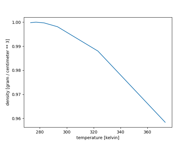
Input > table1  = ((temperature: 273.16, 278.16, 283.16, 293.16, 323.16, 373.16) [kelvin], (density: 0.9998, 1.0000, 0.9997, 0.9981, 0.9880, 0.9583) [gram / centimeter ** 3])

Plot and view datasets

The view statement can be used to display different data structures graphically. This is achieved using the syntax view <mode> (parameter1, paramater2, ...). Two-dimensional datasets can be plotted using lineplot or scatterplot modes. The structure mode is reserved only for AMML structure paramaters from the Atomic and Molecular Modelling Language.

For example, we can use table1 as parameter for the view statement. The data corresponds to the density of liquid water at different temperatures (NIST Chemistry WebBook, Saturation Properties for Water: Liquid Phase Data). When plotting data from a Table, the first parameter of view indicates the dataset’s name, while the second and third parameters point to the “columns” to use for the x and y axes:

Input > view lineplot (table1, 'temperature', 'density')

View plot density of water VS temperature

It is advised to consider the order of evaluation, as the behavior of view can vary depending on execution and evaluation modes.

Models can be recovered, extended, and reused

In an active session, the %uuid magic command will display the model’s Universally Unique Identifier, UUID. As the name indicates, UUIDs are unique for every model. The UUID can be employed for tasks such as recovering, extending, switching, and reusing parts of a model. As an example, displaying the UUID of the current model would return something similar to:

Input > %uuid
uuids: fc2ea86696c441e9afe31c7a9e0745a5 ('fc2ea86696c441e9afe31c7a9e0745a5')

For the sake of this guide, the generic <uuid_of_model_no_1> will be used to further refer to this model.

Starting a new model from the active interactive session

Without exiting the CLI session, it is possible to start a new model, in a new session, by entering the %new magic command. Note that the new session will inherit the options used to start the original session, for example the --auto-run | -r flag. When created, the new model will display its UUID (here simplified for didactic purposes):

Input > %new
Started new session with uuids ('uuid_of_model_no_2')

Recovering and switching models

The UUID can be provided as parameter of the --uuid | -u flag of texts session, which effectively recovers the corresponding model in a new session. This is particularly useful to examine or extend a model any time after closing the session where it was created or processed. For example, recovering the model used to demonstrate data types:

~>$ texts session -r -u <uuid_of_model_no_1>
Input > %hist
COMPLETED  2024-06-26T18:40:13+02:00 str1 = "A string parameter"
COMPLETED  2024-06-26T18:40:18+02:00 bool1 = true
COMPLETED  2024-06-26T18:40:28+02:00 units1 = 2 [seconds]
COMPLETED  2024-06-26T18:40:52+02:00 units2 = 10 [meter] * 3
COMPLETED  2024-06-26T18:40:57+02:00 units3 = units2 / units1
[...]
COMPLETED  2024-06-26T18:38:55+02:00 series1 = (length: 1, 2, 3, 4) [meter]
[...]

Another possibility is to switch between models, without leaving the CLI session, by simply entering the %uuid magic command with a <UUID> as parameter. Since nothing has been added to the second test model, model_no_2, the %hist command will return an empty line:

Input > %uuid <uuid_of_model_no_2>
Input > %hist

Input >

Now we can start populating model_no_2 with some data. For example, two lists with the entropy and enthalpy values of liquid water at the same temperatures from table1:

Input > H = (enthalpy: 1.1021e-05, 0.3794, 0.7578, 1.5125, 3.7721, 7.5522) [kJ / mol]
Input > S = (entropy: -5.3169e-12, 1.3765, 2.7245, 5.3438, 12.682, 23.552 ) [J / mol / K]

Reuse data from other models

If we needed to reuse the temperature data from table1, we would need to inspect, somehow, model_no_1, and then enter the data into model_no_2. In this simple example there is not much complication in doing this manually. However there are many cases where this method would not be adequate, for example when using data from computationally expensive calculations. As a solution the SCL provides the sub-model reuse method, which enables the combination of data from different models. The data copied into the target model preserves all attributes (names, types, parameters, etc.) from the source. The method only requires the name of the original variable and the <UUID> of the source model, for example printing table1 in the new model:

Input > print(table1@<uuid_of_model_no_1>)
Input > %hist
COMPLETED  2024-06-27T15:50:41+02:00 H = (enthalpy: 1.1021e-05, 0.3794, 0.7578, 1.5125, 3.7721, 7.5522) [kJ / mol]
COMPLETED  2024-06-27T15:50:56+02:00 S = (entropy: -5.3169e-12, 1.3765, 2.7245, 5.3438, 12.682, 23.552 ) [J / mol / K]
COMPLETED  2024-06-27T16:16:35+02:00 table1  = ((temperature: 273.16, 278.16, 283.16, 293.16, 323.16, 373.16) [kelvin], (density: 0.9998, 1.0000, 0.9997, 0.9981, 0.9880, 0.9583) [gram / centimeter ** 3])

Expanding your model: operations and functions with data structures

The SCL provides several tools and methods to further expand models, for example by computing new properties from already available data structures, or other objects. These methods include internal functions, operations with series, tables, and arrays, amongst several others described in the documentation.

As an example, we can use the entropy, $S$, enthalpy, $H$, and temperature data (from TempDens) to compute the Gibbs free energy, $G$, of water at different temperatures:

\[G = H - TS\]

The first step is to retrieve the temperature column from the TempDens table:

Input > T = table1.temperature
Input > print(T)
Output > (temperature: 273.16, 278.16, 283.16, 293.16, 323.16, 373.16) [kelvin]

Now that all necessary data is contained in series, we can use the map function to calculate G. The G function is defined employing placeholder variables, which are then mapped to the values in the H, T, and S data series:

Input > G(h, t, s) = h - (t * s)
Input > GibbsE = map(G, H, T, S)
Input > print(GibbsE)
Output > (GibbsE: 1.1021001452364404e-05, -0.003487240000000058, -0.013669420000000043, -0.05408840800000014, -0.3262151200000005, -1.2364643200000005) [kilojoule / mole]

The different series with data of the properties of water can be placed in a new Table data structure, propsH2O, and the change in the Gibbs free energy, G, with respect to the temperature, T can be plotted:

Input > propsH2O = Table (T, H, S, GibbsE)
Input > print(propsH2O)
Output > ((temperature: 273.16, 278.16, 283.16, 293.16, 323.16, 373.16) [kelvin], (enthalpy: 1.1021e-05, 0.3794, 0.7578, 1.5125, 3.7721, 7.5522) [kilojoule / mole], (entropy: -5.3169e-12, 1.3765, 2.7245, 5.3438, 12.682, 23.552) [joule / kelvin / mole], (GibbsE: 1.1021001452364404e-05, -0.003487240000000058, -0.013669420000000043, -0.05408840800000014, -0.3262151200000005, -1.2364643200000005) [kilojoule / mole])
Input > 
Input > view lineplot (propsH2O, 'temperature', 'GibbsE')

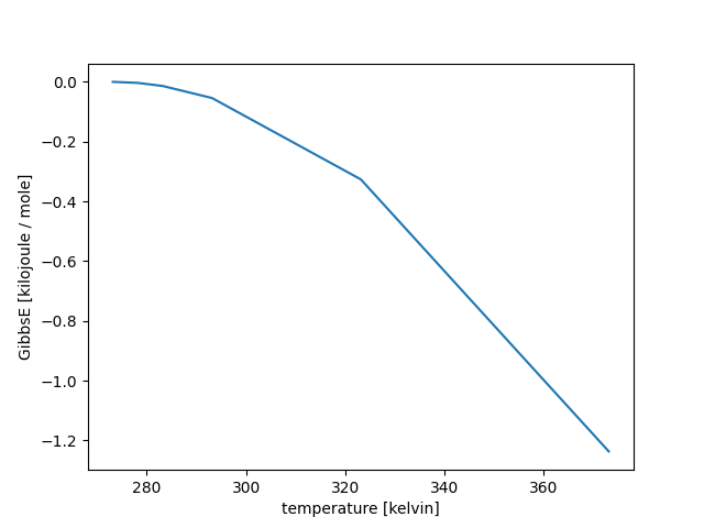
View plot Gibbs free energy of water VS temperature

With the increase in temperature, T, the value of G decreases. This reflects how, for liquid water, transition to vapor phase becomes more favorable as the system is heated.

Enabling more complex models with `texts script`

Model prototyping and testing can benefit greatly from the interactive session, as it provides a quick and simple platform to test variables, functions, data manipulation operations, visualization, and all other methods available for the SCL. Another scenario in which the texts session can be very useful, is to revisit, query, and extend models already in the database.

Nonetheless, due to limitations of its CLI with respect to input and navigation capabilities, the texts session can be impractical in some cases. For example, when building models with large amounts of non-independent steps, or models that require complex input data, such as molecular geometry objects. These models might have nodes that require HPC resources for special calculations, or initricate data structures that need to be passed to other nodes. This is illustrated in this sample model for molecular dynamics simulation. The model requires the setup of several objects such as the molecular structure of the system, the calculators and algorithms to compute the properties of the system, variables and equations for further data manipulation and analysis, and built-in view statements to assist with interpretation of output data.

In this sort of cases, the texts script is a better-suited tool. Here, models are created as independent scripts using available text editors (e.g. vim, nano, etc.), allowing users to exploit the full functionality of these tools. Once ready, the model scripts can be executed in either instant, deferred, or workflow modes, which perform the corresponding syntax and type checks, for example texts script --mode workflow. Concerninig the evaluation of the models:

instant mode will trigger immediate, local, evaluation;
deferred mode evaluation is also local;
workflow mode local evaluation is activated with the --autorun | -r flag.

The script mode also allows the full separation of the execution and evaluation steps, so it is possibile to run the evaluation using texts session after doing, for example, texts script --mode workflow --model-file my_example_model.vm.

To demonstrate how to employ texts script, here a sample recipe to run the molecular dynamics example is provided:

Download the script and the atomic structure file. Make sure to insert the absolute path to the structure filename h2o_box.cif in the second line of the script. Execute the model in workflow mode, -m workflow, indicating the name of the model script --model-file my_file.vm. Without the -r some warnings concerning non-computed data may be printed. These come about due to not computed parameters in view statements.
```
~>$ texts script --mode workflow --model-file Langevin_NVT_H2O.vm
Warning: None:48:16 --> struct.temperature [kelvin] <--
parameter value is not computed yet
Warning: None:51:16 --> rdf <--
parameter value is not computed yet

program UUID: uuid_of_Langevin_md_model
program output: >>>

<<<
```
Use texts session to perform the evaluation of the model, remembering to use the --uuid <uuid_of_my_model> flag to access and update the model already in the database. This step can take a few minutes. Evaluation should be completed once the Input prompt is printed:
```
~>$ texts session -r -u uuid_of_Langevin_md_model
Input >
```
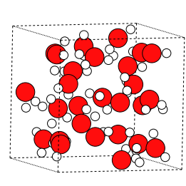
Verify the state of the model using the %hist magic command. The output files from the calculations can be found within the launchdir folders created for the evaluation. Evaluation is finished once all nodes have changed to COMPLETED status.
The view statements in the model script can beused as input to display the different plots. For example the structure of the system after the MD run:
```
Input > view structure (struct)
```

View structure H2O molecular dynamics simulation

Some recommendations on how to run models

Instant and deferred evaluations

Instant and deferred evaluation modes are avilable only in texts script and they are suited for models which can be fully evaluated using local resources. Moreover, the created models are destroyed as soon as texts script returns and not available at later time. To reuse models, and particularly their data, at later time you should consider workflow evaluation mode.

One simple recipe to use instant or deferred modes is:

~>$ texts script --mode [instant|deferred] -f my_model_file.vm

This combination should work for the majority of model scripts under the aforementioned restrictions regarding local resources. The --ignore-warnings | -w flag helps to omit confusing warnings that often come from the packages underlying the VRE Language. Syntax, type, or semantic errors will be caught by the checkers. Evaluation of parameters is triggered by print statements in the models.

Of course, there are some assumptions which help to simplify the choice of flags and options, for example:

the model uses the same grammar version as the grammar provided with the package. Otherwise the --grammar-path | -g flag specifying a path to a compatible grammar is required;
no need for special flags dealing with resources (launchpad and qadapter), which are reserved only for workflow execution;
no debugging, nor special logging options need to be set.

It is advised to run each model script in its own isolated directory to avoid potential clashes due to file read/write operations.

Workflow evaluation

The execution of models in workflow mode is available for both texts script and texts session. It employs a database for data persistence, and allows the use of both local and HPC resources. Workflow execution can require a more hands-on approach, depending on the user’s and model’s requisites.

Depending on the model’s and user’s requirements, workflow evaluation might need additional considerations, compared to instant or deferred modes, leading to a vast number of possibilities to execute such model. Some key points to consider are:

Non-interactive script vs. interactive session

Workflow evaluation is supported for both texts script and texts session. In general, for relatively more intricate models, such as the example shown in this guide, it is advisable to construct the model as an self-contained script, and execute it with texts script -m workflow -f my_model_file.vm. This method triggers no evaluation, but still performs syntax and other checks, while creating the corresponding workflow in the database. Evaluation is independent and can be completed afterwards, for example using

texts script -m workflow -r -u uuid_of_my_model -f my_print_script.vm

with the my_print_script.vm script containing print statements for the desired parameters.

As described earlier, the texts session can be used for testing and fast prototyping models. Other scenarios where session can be a powerful tool are

revisiting models
querying data
extending/reusing models which already exist in the database.

For example, viewing the molecular structure from the example case: texts session -w -r -u uuid_of_Langevin_md_model, followed by view structure(struct). Though possible, texts session is not recommended if the goal is to construct intricate models from the ground.

The texts script and texts session can be used in a combined approach, in which a model is created with a script and then evaluated and inspected using the texts session:

~>$ texts script -m workflow -f my_model.vm
program UUID: uuid_of_my_model
program output: >>>

<<<

~>$ texts session -r -a -u uuid_of_my_model

Input  > print(my_variable1)
Output > sample_output1

Synchronous vs. asynchronous modes

This option is only available in texts session.

By default synchronous mode is selected, which blocks the prompt until all parameters in the model have been evaluated. Synchronous mode is recommended for interactive nodes that run short time. Batch nodes are not processed in this mode.

In contrast, the asynchronous mode performs the evaluation in the background, leaving the prompt ready for further input. Asynchronous mode can be switched on via the --async-run | -a flag, and its use is recommended for evaluation of both batch and interactive nodes.

Absolute vs. relative paths for I/O operations

Files or data read by or exported into a model can be indicated using relative paths with respect to the location of the running script or session. Relative paths work best for interactive nodes, since these are all locally executed and evaluated. Absolute paths should be employed for any models involving batch nodes to avoid any errors during copying or moving data. Though slightly less convenient, absoulte paths are generally recommended to prevent I/O problems.

Also cocerning read/write operations are the launchdir paths. In general, it is advised to allow the creation of unique launchdirs for the evaluation of each individual node, where node-specific output data can be saved. This is the default and can be overriden by the --no-unique-launchdir flag, though some conflicts may occurr if output data, or files, may be overwritten during the evaluation of the model.

Availability of queueing systems (Slurm)

By default, the most standard operations in VRE Language are performed locally on default resources. These are interactive nodes, and are typically evaluated via one process and one thread on one core. Evaluation of interactive nodes can be achieved using either texts script in instant, deferred and workflow modes, or texts session in workflow mode. Since they do not require HPC resources, evaluation can be performed in a local shell, or JupyterLab session. If a database is properly set up, any state updates and output data will be added to the workflow, and will be accessible via the model’s UUID.

The so-called batch nodes, rely on non-local computing resources. These can involve different hardware architectures, software stacks, and queues. The SCL allows specification of these resources via resource annotations. This simple approach enables seamless evaluation of particular statements employing HPC resources. The evaluation of batch nodes is limited to workflow evaluation mode, and can only be performed within HPC clusters that employ scheduling systems such as Slurm. If the resources are not available the interpreter will print an error message indicating “resource exceeds limits” at execution or evaluation times. More details about the use of computational resources for evaluation can be found in here.

Next steps

Learning more

You can continue reading the comprehensive documentation, topic by topic.

Productive use of VRE Language

You can use the comprehensive dicumentation for future reference and features or details that have not been covered in this tutorial. For details about the interpreter, processing modes, and other technical aspects please consult the tools documentation.

Set up a MongoDB database

VRE Language uses FireWorks as workflow management system, which in turn is based on MongoDB database for model persistence. This means that the model will continue to exist in the database, and will be accessible, even after completing its processing. Persistence is achieved only when the interpreter processes a model in workflow evaluation mode.

In this quick-start tutorial, a local file was used to replace the real MongoDB database in order to speedup the setup, and more focus on learning. This local database feature is recommended only for testing and learning purposes. For production purposes, such as using VRE Language on a computing cluster, in the cloud etc., you will have to set up a MongoDB database. Therefore, you need to run a local MongoDB instance or use a MongoDB service from your computing center or some cloud provider. For detailed instructions, see e.g. this installation guide.